Anomaly detection

An anomaly in OpenSearch is any unusual behavior change in your time-series data. Anomalies can provide valuable insights into your data. For example, for IT infrastructure data, an anomaly in the memory usage metric can help identify early signs of a system failure.

Conventional techniques like visualizations and dashboards can make it difficult to uncover anomalies. Configuring alerts based on static thresholds is possible, but this approach requires prior domain knowledge and may not adapt to data with organic growth or seasonal trends.

Anomaly detection automatically detects anomalies in your OpenSearch data in near real time using the Random Cut Forest (RCF) algorithm. RCF is an unsupervised machine learning algorithm that models a sketch of your incoming data stream to compute an anomaly grade and confidence score value for each incoming data point. These values are used to differentiate an anomaly from normal variations. For more information about how RCF works, see Robust Random Cut Forest Based Anomaly Detection on Streams.

You can pair the Anomaly Detection plugin with the Alerting plugin to notify you as soon as an anomaly is detected.

Getting started with anomaly detection in OpenSearch Dashboards

To get started, go to OpenSearch Dashboards > OpenSearch Plugins > Anomaly Detection.

Step 1: Define a detector

A detector is an individual anomaly detection task. You can define multiple detectors, and all detectors can run simultaneously, with each analyzing data from different sources. You can define a detector by following these steps:

1. On the Anomaly detection page, select the Create detector button.

2. On the Define detector page, add the detector details. Enter a name and a brief description. The name must be unique and descriptive enough to help you identify the detector’s purpose.

3. In the Select data pane, specify the data source by selecting one or more sources from the Index dropdown menu. You can select indexes, index patterns, or aliases.

   • Detectors can use remote indexes, which you can access using the cluster-name:index-name pattern. For more information, see Cross-cluster search. Starting in OpenSearch Dashboards 2.17, you can also select clusters and indexes directly. If the Security plugin is enabled, see Selecting remote indexes with fine-grained access control in the Anomaly detection security documentation.

   • To create a cross-cluster detector in OpenSearch Dashboards, you must have the following permissions: indices:data/read/field_caps, indices:admin/resolve/index, and cluster:monitor/remote/info.

4. (Optional) Filter the data source by selecting Add data filter and then specifying the conditions for Field, Operator, and Value. Alternatively, select Use query DSL and enter your filter as a JSON-formatted Boolean query. Only Boolean queries are supported for query domain-specific language (DSL).

Example: Filtering data using query DSL

The following example query retrieves documents in which the urlPath.keyword field matches any of the specified values:

 {
    "bool": {
       "should": [
             {
                "term": {
                   "urlPath.keyword": "/domain/{id}/short"
                }
             },
             {
                "term": {
                   "urlPath.keyword": "/sub_dir/{id}/short"
                }
             },
             {
                "term": {
                   "urlPath.keyword": "/abcd/123/{id}/xyz"
                }
             }
       ]
    }
 }

1. In the Timestamp pane, select a field from the Timestamp field dropdown list.

2. (Optional) To store anomaly detection results in a custom index, select Enable custom results index and provide a name for your index (for example, abc). The plugin creates an alias prefixed with opensearch-ad-plugin-result- followed by your chosen name (for example, opensearch-ad-plugin-result-abc). This alias points to an actual index with a name containing the date and a sequence number, such as opensearch-ad-plugin-result-abc-history-2024.06.12-000002, where your results are stored.

You can use - to separate the namespace to manage custom results index permissions. For example, if you use opensearch-ad-plugin-result-financial-us-group1 as the results index, you can create a permission role based on the pattern opensearch-ad-plugin-result-financial-us-* to represent the financial department at a granular level for the us group.

Permissions

When the Security plugin (fine-grained access control) is enabled, the default results index becomes a system index and is no longer accessible through the standard Index or Search APIs. To access its content, you must use the Anomaly Detection RESTful API or the dashboard. As a result, you cannot build customized dashboards using the default results index if the Security plugin is enabled. However, you can create a custom results index in order to build customized dashboards.

If the custom index you specify does not exist, the Anomaly Detection plugin will create it when you create the detector and start your real-time or historical analysis.

If the custom index already exists, the plugin will verify that the index mapping matches the required structure for anomaly results. In this case, ensure that the custom index has a valid mapping as defined in the anomaly-results.json file. To use the custom results index option, you must have the following permissions:

• indices:admin/create – The create permission is required in order to create and roll over the custom index.
• indices:admin/aliases – The aliases permission is required in order to create and manage an alias for the custom index.
• indices:data/write/index – The write permission is required in order to write results into the custom index for a single-entity detector.
• indices:data/read/search – The search permission is required in order to search custom results indexes to show results on the Anomaly Detection interface.
• indices:data/write/delete – The detector may generate many anomaly results. The delete permission is required in order to delete old data and save disk space.
• indices:data/write/bulk* – The bulk* permission is required because the plugin uses the Bulk API to write results into the custom index.

Flattening nested fields

Custom results index mappings with nested fields pose aggregation and visualization challenges. The Enable flattened custom result index option flattens the nested fields in the custom results index. When selecting this option, the plugin creates a separate index prefixed with the custom results index name and detector name. For example, if the detector Test uses the custom results index abc, a separate index with the alias opensearch-ad-plugin-result-abc-flattened-test will store the anomaly detection results with nested fields flattened.

In addition to creating a separate index, the plugin also sets up an ingest pipeline with a script processor. This pipeline is bound to the separate index and uses a Painless script to flatten all nested fields in the custom results index.

Deactivating this option on a running detector removes its flattening ingest pipeline; it also ceases to be the default for the results index. When using the flattened custom result option, consider the following:

• The Anomaly Detection plugin constructs the index name based on the custom results index and detector name, and because the detector name is editable, conflicts can occur. If a conflict occurs, the plugin reuses the index name.
• When managing the custom results index, consider the following:
  • The Anomaly Detection dashboard queries all detector results from all custom results indexes. Having too many custom results indexes can impact the plugin’s performance.
  • You can use Index State Management to roll over old results indexes. You can also manually delete or archive any old results indexes. Reusing a custom results index for multiple detectors is recommended.

The plugin rolls over an alias to a new index when the custom results index meets any of the conditions in the following table.

After defining your detector settings, select Next to configure the model.

Step 2: Configure the model

Add features to your detector. A feature is an aggregation of a field or a Painless script. A detector can discover anomalies across one or more features.

You must choose an aggregation method for each feature: average(), count(), sum(), min(), or max(). The aggregation method determines what constitutes an anomaly. For example, if you choose min(), the detector focuses on finding anomalies based on the minimum values of your feature. If you choose average(), the detector finds anomalies based on the average values of your feature.

You can also use custom JSON aggregation queries as an aggregation method. For more information about creating JSON aggregation queries, see Query DSL.

For each configured feature, you can also select the anomaly criteria. By default, the model detects an anomaly when the actual value is either abnormally higher or lower than the expected value. However, you can customize your feature settings so that anomalies are only registered when the actual value is higher than the expected value (indicating a spike in the data) or lower than the expected value (indicating a dip in the data). For example, when creating a detector for the cpu_utilization field, you may choose to register anomalies only when the value spikes in order to reduce alert fatigue.

Suppressing anomalies with threshold-based rules

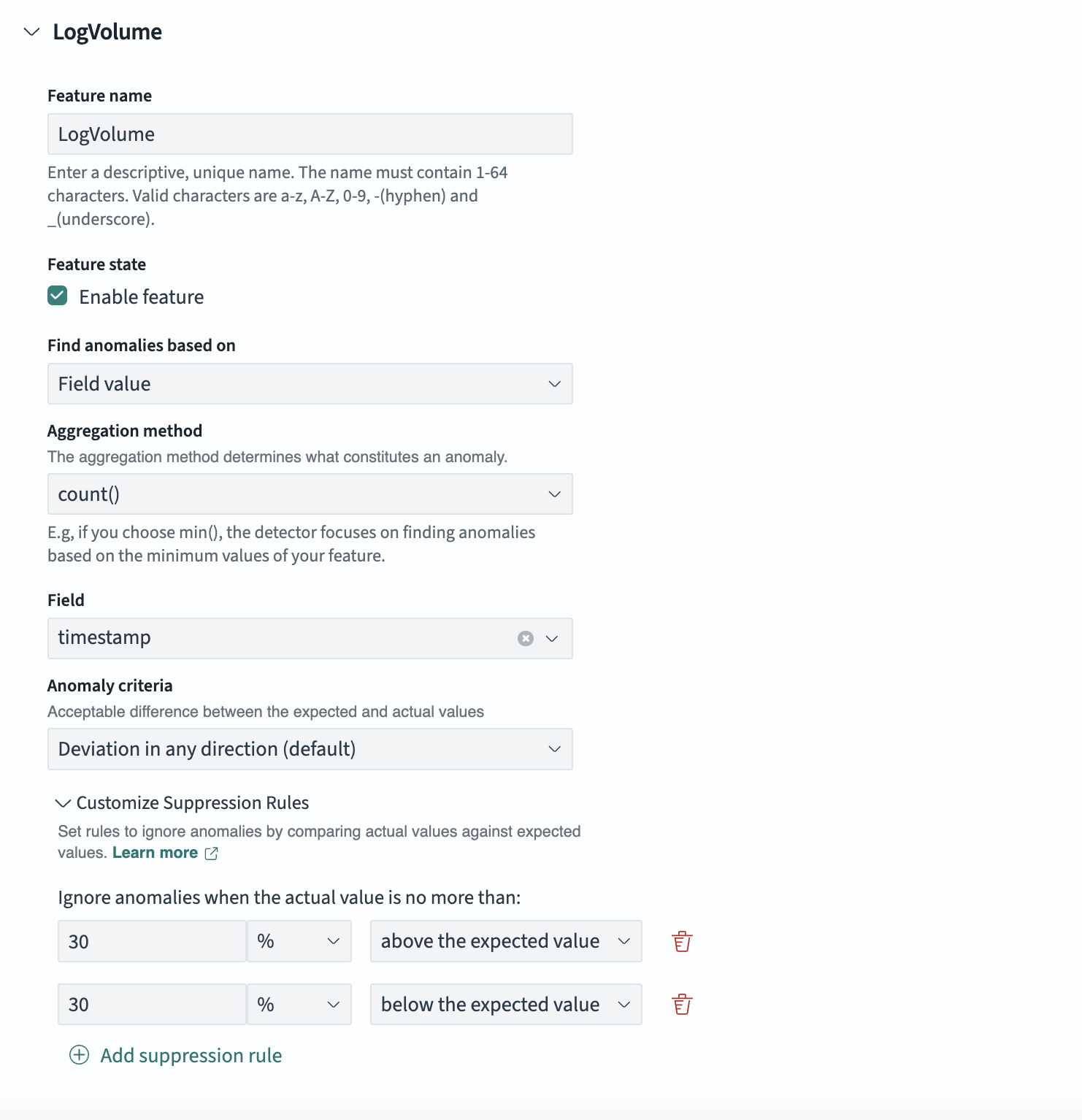
In the Feature selection pane, you can suppress anomalies by setting rules that define acceptable differences between the expected and actual values, either as an absolute value or a relative percentage. This helps reduce false anomalies caused by minor fluctuations, allowing you to focus on significant deviations.

To suppress anomalies for deviations of less than 30% from the expected value, you can set the following rules in the feature selection pane:

• Ignore anomalies when the actual value is no more than 30% above the expected value.
• Ignore anomalies when the actual value is no more than 30% below the expected value.

The following image shows the pane for a feature named LogVolume, where you can set the relative deviation percentage settings:

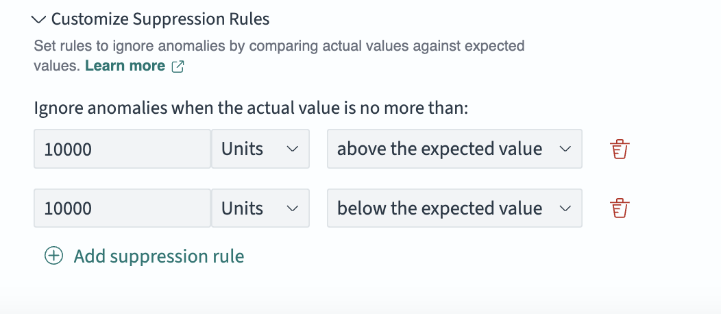
If you expect that the log volume should differ by at least 10,000 from the expected value before being considered an anomaly, you can set the following absolute thresholds:

• Ignore anomalies when the actual value is no more than 10,000 above the expected value.
• Ignore anomalies when the actual value is no more than 10,000 below the expected value.

The following image shows the pane for a feature named LogVolume, where you can set the absolute threshold settings:

If no custom suppression rules are set, then the system defaults to a filter that ignores anomalies with deviations of less than 20% from the expected value for each enabled feature.

A multi-feature model correlates anomalies across all of its features. The curse of dimensionality makes it less likely that a multi-feature model will identify smaller anomalies as compared to a single-feature model. Adding more features can negatively impact the precision and recall of a model. A higher proportion of noise in your data can further amplify this negative impact. To select the optimal feature set limit for anomalies, we recommend an iterative process of testing different limits. By default, the maximum number of features for a detector is 5. To adjust this limit, use the plugins.anomaly_detection.max_anomaly_features setting.

Configuring a model based on an aggregation method

To configure an anomaly detection model based on an aggregation method, follow these steps:

1. On the Detectors page, select the desired detector from the list.
2. On the detector’s details page, select the Actions button to activate the dropdown menu and then select Edit model configuration.
3. On the Edit model configuration page, select the Add another feature button.
4. Enter a name in the Feature name field and select the Enable feature checkbox.
5. Select Field value from the dropdown menu under Find anomalies based on.
6. Select the desired aggregation from the dropdown menu under Aggregation method.
7. Select the desired field from the options listed in the dropdown menu under Field.
8. Select the Save changes button.

Configuring a model based on a JSON aggregation query

To configure an anomaly detection model based on a JSON aggregation query, follow these steps:

1. On the Edit model configuration page, select the Add another feature button.
2. Enter a name in the Feature name field and select the Enable feature checkbox.
3. Select Custom expression from the dropdown menu under Find anomalies based on. The JSON editor window will open.
4. Enter your JSON aggregation query in the editor.
5. Select the Save changes button.

For acceptable JSON query syntax, see OpenSearch Query DSL.

Setting categorical fields for high cardinality

You can categorize anomalies based on a keyword or IP field type. You can enable the Categorical fields option to categorize, or “slice,” the source time series using a dimension, such as an IP address, a product ID, or a country code. This gives you a granular view of anomalies within each entity of the category field to help isolate and debug issues.

To set a category field, select Enable categorical fields and select a field. You cannot change the category fields after you create the detector.

Only a certain number of unique entities are supported in the category field. Use the following equation to calculate the recommended total number of entities supported in a cluster:

(data nodes * heap size * anomaly detection maximum memory percentage) / (entity model size of a detector)

To get the detector’s entity model size, use the Profile Detector API. You can adjust the maximum memory percentage using the plugins.anomaly_detection.model_max_size_percent setting.

Consider a cluster with 3 data nodes, each with 8 GB of JVM heap size and the default 10% memory allocation. With an entity model size of 1 MB, the following formula calculates the estimated number of unique entities:

(8096 MB * 0.1 / 1 MB ) * 3 = 2429

If the actual total number of unique entities is higher than the number that you calculate (in this case, 2,429), then the anomaly detector attempts to model the extra entities. The detector prioritizes both entities that occur more often and are more recent.

This formula serves as a starting point. Make sure to test it with a representative workload. See the OpenSearch blog post Improving Anomaly Detection: One million entities in one minute for more information.

Operational settings

The Suggest parameters button in OpenSearch Dashboards initiates a review of recent history in order to recommend sensible defaults. You can override these defaults by adjusting the following parameters.

Detector interval

Specifies the aggregation bucket size (for example, 10 minutes). You should set the detector interval based on your actual data characteristics:

• Longer intervals: Smooth out noise and reduce compute costs but delay detection.
• Shorter intervals: Detect changes sooner but increase resource usage and can introduce noise.

The interval must be large enough that you rarely miss data. The model uses shingling (consecutive, contiguous buckets), and missing buckets degrade data quality and shingle formation.

Frequency (Optional)

Specifies how often the job queries, scores, and writes results. Shorter values provide more real-time updates at a higher cost, while longer values reduce load but slow down updates. Frequency must be a multiple of the interval and defaults to the interval value.

If you’re unsure, leave this field blank—the job will use the interval value by default.

Common scenarios for using a larger frequency than the interval include:

1. Batching short buckets for efficiency: In high-frequency or high-volume log streams where ultra-fast alerting is unnecessary. For workloads with heavy joins or high-cardinality features, or for compliance-driven nightly rollups that require an immutable daily anomaly ledger for reviews or audits, running the detector every 1–2 minutes can be wasteful. Instead, schedule the detector to run less frequently so it batches many short intervals in one pass (for example, 6 hours, which processes ~360 1-minute buckets at once). Choose a frequency that fits your alerting latency and cost goals (for example, 30 minutes, 1 hour, 3 hours, 6 hours, or 12 hours).

• Benefits: Reduced scheduling overhead and better resource utilization, especially when running many jobs or working with busy clusters.
• Trade-offs: Increased detection delay—an anomaly in a 1-minute bucket may only be reported when the batch run is executed.
• Best for: Cost and load control, compliance and audit.

1. Aligning with infrequent or batch log ingestion: When logs arrive irregularly or in batches (for example, once per day from S3, or IoT devices that upload in bursts). Running the detector every minute would mostly yield empty results and wasted cycles. Configure the frequency closer to the data arrival rate (for example, 1 day) so each search is more likely to find new data. When timestamps are irregular and low in volume (as is common with sporadic logs), interim results tend to be harmful to accuracy, as the RCF model is stateful and assumes strict ascending order of timestamps. By using a less frequent schedule, you effectively let the job wait for complete data rather than repeatedly checking an empty index.

   • Benefits: Reduced pointless queries and CPU overhead; improved efficiency and more accurate results—anomalies will be evaluated once the batch of logs arrives, with minimal risk of false interim anomalies.
   • Trade-offs: Less frequent anomaly evaluation.
   • Best for: Batch jobs and sporadic log ingestion patterns.

Window delay (Optional)

To add extra processing time for data collection, specify a Window delay value. This signals to the detector that data is not ingested into OpenSearch in real time but with a certain delay.

How it works:

Set the window delay to shift the detector interval to account for ingestion delay. For example:

• Detector interval: 10 minutes
• Data ingestion delay: 1 minute
• Detector runs at: 2:00 PM

Without a window delay, the detector attempts to get data from 1:50–2:00 PM but only gets 9 minutes of data, missing data from 1:59–2:00 PM. Setting the window delay to 1 minute shifts the interval window to 1:49–1:59 PM, ensuring the detector captures all 10 minutes of data.

Best practices:

• Set Window delay to the upper limit of expected ingestion delay to avoid missing data.
• Balance data accuracy with timely detection—too long of a delay hinders real-time anomaly detection.

History (Optional)

Sets the number of historical data points used to train the initial (cold-start) model. The maximum is 10,000 data points. More history improves initial model accuracy up to that limit.

Choosing between frequency and window delay

Both frequency and window delay address ingestion delay but work better for different data patterns:

• Window delay: Best for streaming data (continuous trickle)
• Frequency: Best for batch data (periodic drops)

Example scenarios:

• Example A – Data arrives every minute, but always 1 day late → use window delay:
  • Pattern: Data for Day-1 00:01, 00:02, ..., 23:59 arrives steadily, but only on Day-2 at the same minute marks.
  • Configuration: interval = 1 min, window_delay = 1 day, frequency = 1 min.
  • Effect:
    • The Day-2 00:01 run processes Day-1 00:01 data.
    • The Day-2 00:02 run processes Day-1 00:02 data.
    • …
    • The Day-2 23:59 run processes Day-1 23:59 data.
  • Why this fits: Each minute’s data arrives with a predictable 24-hour delay. Setting a 1-day window delay ensures each record is processed at its intended timestamp while keeping the workload incremental.
• Example B – All of Day-1’s data arrives at Day-2 00:00 → use a daily frequency:
  • Pattern: No data appears during Day-1; instead, a single batch containing all 1,440 minutes of data arrives at Day-2 00:00.
  • Configuration: interval = 1 min, frequency = 1 day (process the full day at once). (Tip: Add a small window_delay—for example, 1–5 minutes—to account for indexing or refresh lag.)
  • Effect:
    • Best case: If the detector starts around 00:00, the Day-2 00:00 run processes all of Day-1’s data right after it arrives.
    • Worst case: If the detector starts around 23:59, the daily run won’t occur until Day-2 23:59, roughly 24 hours after the drop.
    • General rule: For a midnight data drop, the extra wait equals your detector’s daily start time.
  • Why this works: Because the entire day’s data becomes available at once, a single daily run is much more efficient than processing data minute by minute.

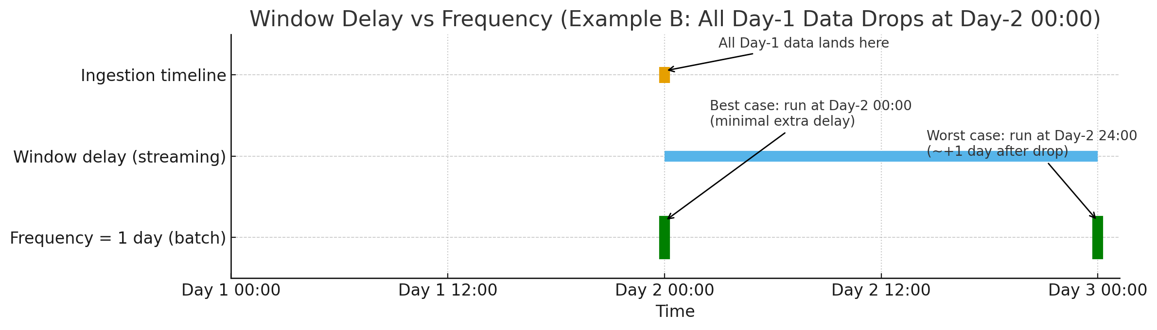
The following diagram illustrates the timing differences between using window delay and using frequency to handle a 1-day ingestion delay. The timeline shows Day-1 ingestion (top), Day-2 processing with window_delay = 1 day (middle, continuous band), and a single daily run when frequency = 1 day (bottom, vertical bar). Depending on when you start the detector, a daily frequency can fire just after Day-1 ends (best case, minimal extra delay) or much later (worst case, up to ~+1 day). The job runs every day at approximately the time you first started it.

Setting a shingle size

In the Advanced settings pane, you can set the number of data stream aggregation intervals to include in the detection window. Choose this value based on your actual data to find the optimal setting for your use case. To set the shingle size, select Show in the Advanced settings pane. Enter the desired size in the intervals field.

The anomaly detector requires the shingle size to be between 1 and 128. The default is 8. Use 1 only if you have at least two features. Values of less than 8 may increase recall but also may increase false positives. Values greater than 8 may be useful for ignoring noise in a signal.

Setting an imputation option

In the Advanced settings pane, you can set the imputation option. This allows you to manage missing data in your streams. The options include the following:

• Ignore Missing Data (Default): The system continues without considering missing data points, keeping the existing data flow.
• Fill with Custom Values: Specify a custom value for each feature to replace missing data points, allowing for targeted imputation tailored to your data.
• Fill with Zeros: Replace missing values with zeros. This is ideal when the absence of data indicates a significant event, such as a drop to zero in event counts.
• Use Previous Values: Fill gaps with the last observed value to maintain continuity in your time-series data. This method treats missing data as non-anomalous, carrying forward the previous trend.

Using these options can improve recall in anomaly detection. For instance, if you are monitoring for drops in event counts, including both partial and complete drops, then filling missing values with zeros helps detect significant data absences, improving detection recall.

Be cautious when imputing extensively missing data, as excessive gaps can compromise model accuracy. Quality input is critical—poor data quality leads to poor model performance. The confidence score also decreases when imputations occur. You can check whether a feature value has been imputed using the feature_imputed field in the anomaly results index. See Anomaly result mapping for more information.

Previewing sample anomalies

You can preview anomalies based on sample feature input and adjust the feature settings as needed. The Anomaly Detection plugin selects a small number of data samples—for example, 1 data point every 30 minutes—and uses interpolation to estimate the remaining data points to approximate the actual feature data. The sample dataset is loaded into the detector, which then uses the sample dataset to generate a preview of the anomalies.

1. Select Preview sample anomalies.
   • If sample anomaly results are not displayed, check the detector interval to verify that 400 or more data points are set for the entities during the preview date range.
2. Select the Next button.

Step 3: Set up detector jobs

To start a detector to find anomalies in your data in near real time, select Start real-time detector automatically (recommended).

Alternatively, if you want to perform historical analysis and find patterns in longer historical data windows (weeks or months), select the Run historical analysis detection box and select a date range of at least 128 detection intervals.

Analyzing historical data can help to familiarize you with the Anomaly Detection plugin. For example, you can evaluate the performance of a detector against historical data in order to fine-tune it.

You can experiment with historical analysis by using different feature sets and checking the precision before using real-time detectors.

Step 4: Review detector settings

Review your detector settings and model configurations to confirm that they are valid and then select Create detector.

If a validation error occurs, edit the settings to correct the error and return to the detector page.

Step 5: Observe the results

Select either the Real-time results or Historical analysis tab. For real-time results, it will take some time to display the anomaly results. For example, if the detector interval is 10 minutes, then the detector may take an hour to initiate because it is waiting for sufficient data to be able to generate anomalies.

A shorter interval results in the model passing the shingle process more quickly and generating anomaly results sooner. You can use the profile detector operation to ensure that you have enough data points.

If the detector is pending in “initialization” for longer than 1 day, aggregate your existing data and use the detector interval to check for any missing data points. If you find many missing data points, consider increasing the detector interval.

Click and drag over the anomaly line chart to zoom in and see a detailed view of an anomaly.

You can analyze anomalies using the following visualizations:

• Live anomalies (for real-time results) displays live anomaly results for the last 60 intervals. For example, if the interval is 10, it shows results for the last 600 minutes. The chart refreshes every 30 seconds.
• Anomaly overview (for real-time results) or Anomaly history (for historical analysis on the Historical analysis tab) plot the anomaly grade with the corresponding measure of confidence. The pane includes:
  • The number of anomaly occurrences based on the given data-time range.
  • The Average anomaly grade, a number between 0 and 1 that indicates how anomalous a data point is. An anomaly grade of 0 represents “not an anomaly,” and a non-zero value represents the relative severity of the anomaly.
  • Confidence estimate of the probability that the reported anomaly grade matches the expected anomaly grade. Confidence increases as the model observes more data and learns the data behavior and trends. Note that confidence is distinct from model accuracy.
  • Last anomaly occurrence is the time at which the last anomaly occurred.

The following sections can be found under Anomaly overview and Anomaly history:

• Feature breakdown plots the features based on the aggregation method. You can vary the date-time range of the detector. Selecting a point on the feature line chart shows the Feature output, the number of times a field appears in your index, and the Expected value, a predicted value for the feature output. Where there is no anomaly, the output and expected values are equal.

• Anomaly occurrences shows the Start time, End time, Data confidence, and Anomaly grade for each detected anomaly. To view logs related to an occurrence in Discover, select the View in Discover icon in the Actions column. The logs include a 10-minute buffer before and after the start and end times.

Selecting a point on the anomaly line chart shows Feature Contribution, the percentage of a feature that contributes to the anomaly

If you set the category field, you see an additional Heat map chart. The heat map correlates results for anomalous entities. This chart is empty until you select an anomalous entity. You also see the anomaly and feature line chart for the time period of the anomaly (anomaly_grade > 0).

If you have set multiple category fields, you can select a subset of fields to filter and sort the fields by. Selecting a subset of fields lets you see the top values of one field that share a common value with another field.

For example, if you have a detector with the category fields ip and endpoint, you can select endpoint in the View by dropdown menu. Then select a specific cell to overlay the top 20 values of ip on the charts. The Anomaly Detection plugin selects the top ip by default. You can see a maximum of 5 individual time-series values at the same time.

Step 6: Set up alerts

Under Real-time results, select Set up alerts and configure a monitor to notify you when anomalies are detected. For instructions on how to create a monitor and set up notifications based on your anomaly detector, see Configuring anomaly alerting.

If you stop or delete a detector, make sure to delete any monitors associated with it.

Viewing and updating the detector configuration

To view all the configuration settings for a detector, select the Detector configuration tab.

1. To make any changes to the detector configuration or fine-tune the time interval to minimize any false positives, go to the Detector configuration section and select Edit. You must stop real-time and historical analysis to change the detector’s configuration. Confirm that you want to stop the detector and proceed.
2. To enable or disable features, in the Features section, select Edit and adjust the feature settings as needed. After you make your changes, select Save and start detector.

Managing your detectors

To start, stop, or delete a detector, go to the Detectors page.

1. Select the detector name.
2. Select Actions and then select Start real-time detectors, Stop real-time detectors, or Delete detectors.

Related articles

• Anomaly detection API
• Settings
• Anomaly result mapping
• Anomaly detection security
• Anomaly detection visualizations and dashboards
• Configuring anomaly alerting