Data table

A data table displays selected fields in row-column form. You can display one or more metrics as columns, bucketed into rows, and subdivide bucket data into separate tables.

When to use data tables

Use data tables to examine individual documents, verify data quality, or investigate details behind aggregate visualizations. You can sort, filter, and examine correlations between fields that might not be apparent in more abstract visualizations. Use data tables as drill-down targets to move from high-level visual summaries to specific record-level details.

Creating a data table

The examples on this page use the Sample flight data dataset. Before you begin, complete the prerequisites.

To create a data table, follow these steps:

1. In the New Visualization dialog, select Data Table, then select your index pattern (for example, opensearch_dashboards_sample_data_flights).

   By default, the visualization selects Count as the only metric to display. Since the data is not bucketed, it displays the total document count.

   For this dataset the count is 13,059 if none of the data has been filtered out. If your visualization displays a different value, make sure that your time filter window is large enough to encompass all the sample flight data. See time filter.

2. In the Metrics panel, expand Metric Count.
3. Set Aggregation to Average and Field to FlightDelayMin.
4. (Optional) Enter a Custom label, for example Flight delay in minutes.

5. Select Update.

   The table displays a single value for all the data, 47.335. This is the average flight delay for every document in the flight database, including zero-minute delays.

6. In the Buckets panel, select Add > Split rows.
7. Set Aggregation to Terms and Field to FlightDelay.

8. Select Update.

   The table shows that non-delayed flights averaged zero minutes of delay time. The nonzero flight delay bucket is considerably higher than the overall value because the zero delays are no longer part of that average.

9. Change the row buckets by choosing Range from the Aggregation dropdown and DistanceMiles from the Field dropdown.

10. Configure the following ranges (select Add range for the third row):

    From	To
    0	4000
    4000	8000
    8000	Infinity

11. In the Metrics panel, select Add > Metric and set Aggregation to Count.

    Select Add in the Metrics panel, not the Buckets panel.

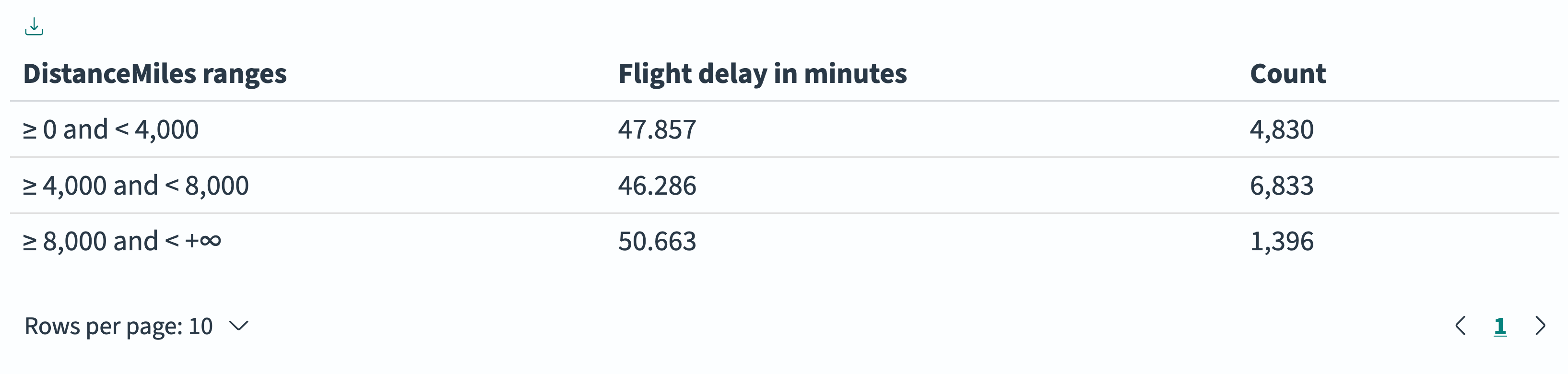
12. Select Update.

    The table shows the average flight delay and count for each distance range, as shown in the following image.

    

Displaying multiple columns

A data table always includes at least one metric. When the Metrics panel contains a single metric, the panel provides no option to remove or disable it, so an aggregation-based data table cannot be built without a metric column. To display several columns, add a bucket or a Top Hit metric for each field.

Adding a column for each field you group by

Each Split rows bucket adds a column to the table.

This example starts from a new data table that uses the default Count metric. If you continue from the previous procedure, the table retains the DistanceMiles bucket and both metrics, so it displays additional columns.

To group flights by carrier and destination country, follow these steps:

1. In the Buckets panel, select Add > Split rows.
2. Set Aggregation to Terms and Field to Carrier.
3. Select Add > Split rows a second time.
4. Set Aggregation to Terms and Field to DestCountry.
5. Select Update.

The table displays three columns: Carrier: Descending, DestCountry: Descending, and the metric column. A bucket column is labeled with the field name and the sort order of the bucket. The buckets are nested, so each row pairs one carrier with one of the destination countries that appears in its documents.

Adding a column of field values

The Top Hit metric returns a value taken directly from a document, and in a data table it accepts string fields as well as numeric ones. Each Top Hit metric becomes a column of field values. To add the destination city of each group’s most recent flight, follow these steps:

1. In the Metrics panel, select Add > Metric.
2. From the Aggregation dropdown list, select Top Hit.
3. From the Field dropdown list, select DestCityName.
4. Verify that Size is set to 1, Sort on is set to timestamp, and Order is set to Descending.
5. Select Update.

The table now displays four columns: Carrier: Descending, DestCountry: Descending, Count, and Last DestCityName. Each row reports how many flights the carrier operated to that country and the city where its most recent flight landed, such as Rome or San Antonio. To add a column for each additional field, repeat these steps and select a different field.

Top Hit returns values from the documents in each row’s bucket, so the table still groups documents. Raising Size returns that many values in one cell, but the documents in a bucket often repeat the same value, so the cell lists one city many times. To give each document its own row, see Listing individual documents.

Listing individual documents

To build a table in which each row is a single document and each column is a field, save a search in the Discover application instead of creating a data table. Discover returns documents without aggregating them, and a saved search can be added to a dashboard in the same Add panels dialog as a visualization.

To choose which fields appear as columns, see Using the field select tool. To place the saved search on a dashboard, see Adding a visualization to a dashboard.

Configuring a data table

For information about general visualization configuration, see Configuring visualizations.

Next steps

• To choose a different visualization type, see Visualization types.
• To add this visualization to a dashboard, see Creating dashboards.