Timeline visualizations
Timeline is an expression-based data visualization tool in OpenSearch Dashboards that you can use to create time-series visualizations using a simple expression language. Unlike other visualization types that use a graphical interface, Timeline uses a text-based expression syntax to define data sources, transformations, and display options. With this syntax, you can compare multiple time series, apply mathematical functions, and overlay data from different time periods.
When to use timeline visualizations
Use Timeline for exclusively time-based data analysis, particularly for revealing temporal patterns and event sequences using its expression syntax.
Timeline is a legacy visualization tool. For new time-based visualizations, consider using TSVB or Vega.
Timeline is best suited for scenarios where you need expression-based control over your visualizations, such as comparing data across time periods using offsets, applying mathematical transformations to series, or combining multiple data sources on a single chart.
Prerequisites
Before creating a timeline visualization, ensure that you have the following:
- An OpenSearch Dashboards instance running and accessible.
- Sample data loaded or a time-series index available. The examples in this document use the e-commerce sample dataset. To learn about adding sample datasets, see Adding sample data.
Creating a timeline visualization
To create a timeline visualization, follow these steps:
- From the top menu, select OpenSearch Dashboards > Visualize.
- Select Create visualization.
- Select Timeline.
The timeline editor consists of the following components:
- Chart area: Displays the rendered visualization.
- Interval: Sets the time bucket size for data aggregation (for example,
1d,1h, orauto). - Timeline expression: The text editor where you write timeline expressions to define the data and appearance of your visualization.
- Update and Discard buttons: Apply or revert changes to the expression.
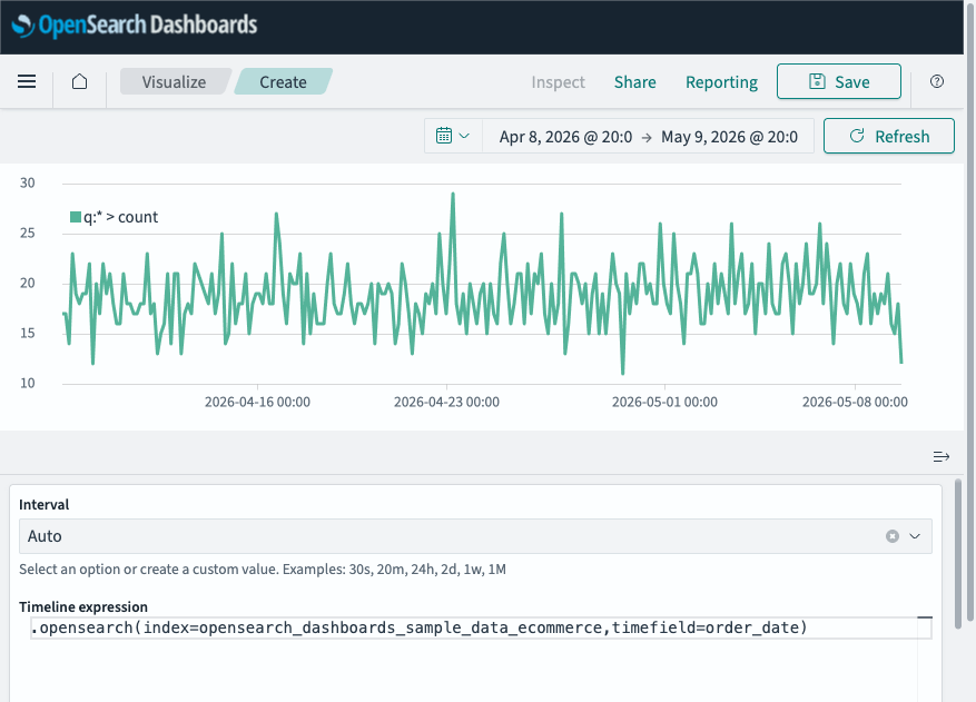
The following image shows the timeline editor containing a basic expression that queries e-commerce data.
Timeline expression syntax
A timeline expression consists of one or more function chains separated by commas. Each chain starts with a data source function and is followed by additional functions chained using dot notation. Multiple chains are separated by commas and produce multiple series on the same chart.
The basic syntax is as follows:
.function1(arg1=value1, arg2=value2).function2(arg1=value1)
To display multiple series on the same chart, separate the expressions with commas:
.opensearch(index=my-index).label("Series 1"), .opensearch(index=my-index, metric=avg:price).label("Series 2")
Data source functions
The .opensearch() function is the primary data source for timeline expressions. It pulls time-series data from an OpenSearch index.
.opensearch() parameters
The following table lists the .opensearch() function parameters.
| Parameter | Type | Description |
|---|---|---|
q | String | A query in Apache Lucene query string syntax. Default is * (match all). |
metric | String | An OpenSearch metric aggregation: avg, sum, min, max, percentiles, or cardinality, followed by a field name. For example, sum:bytes or percentiles:bytes:95,99,99.9. Default is count. |
split | String | A field on which to split the series and a limit. For example, hostname:10 retrieves the top 10 hostnames. |
index | String | The index to query. Wildcards are accepted. Provide an index pattern name for scripted fields and field name suggestions. |
timefield | String | A field of type date to use for the x-axis. |
offset | String | Offsets the series retrieval by a date expression, for example, -1M to make events from one month ago appear as if they are happening now. Use timerange:-2 to offset by twice the overall chart time range to the past. |
opensearchDashboards | Boolean | When set to true, respects filters applied on OpenSearch Dashboards dashboards. Only has an effect when used on dashboards. |
data_source_name | String | The data source to query from. Only works when multiple data sources are enabled. |
fit | String | The algorithm to use for fitting series to the target time span and interval. One of average, carry, nearest, none, or scale. |
Basic query example
The following expression retrieves a count of documents from the e-commerce sample data index over time:
.opensearch(index=opensearch_dashboards_sample_data_ecommerce, timefield=order_date)
Metric aggregation example
The following expression calculates the average value of the taxful_total_price field:
.opensearch(index=opensearch_dashboards_sample_data_ecommerce, timefield=order_date, metric=avg:taxful_total_price)
Query filter example
The following expression uses the q parameter to filter data using Lucene query syntax:
.opensearch(index=opensearch_dashboards_sample_data_ecommerce, timefield=order_date, q="customer_gender:MALE").label("Male Orders"),
.opensearch(index=opensearch_dashboards_sample_data_ecommerce, timefield=order_date, q="customer_gender:FEMALE").label("Female Orders")
Split example
The following expression splits the data by the customer_gender field, returning the top 2 values:
.opensearch(index=opensearch_dashboards_sample_data_ecommerce, timefield=order_date, split=customer_gender:2)
Offset example
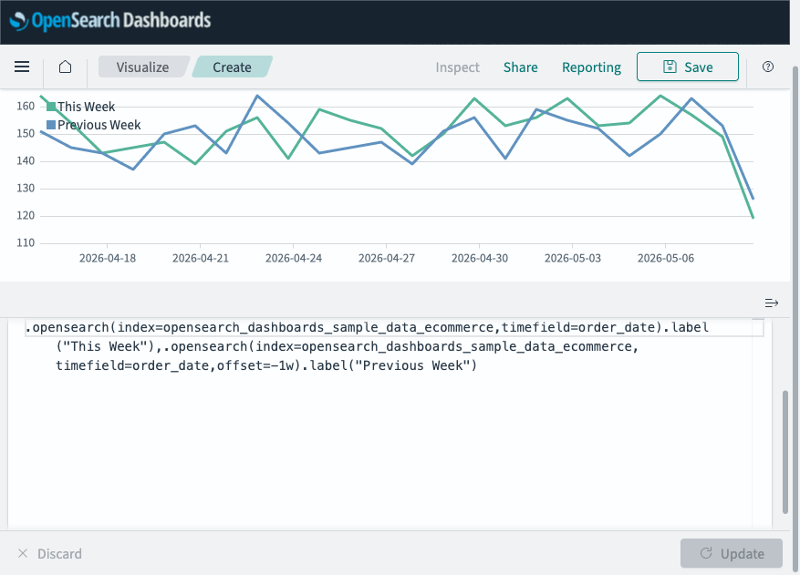
The following expression overlays the current time range with data from one week ago for comparison:
.opensearch(index=opensearch_dashboards_sample_data_ecommerce, timefield=order_date).label("This Week"),
.opensearch(index=opensearch_dashboards_sample_data_ecommerce, timefield=order_date, offset=-1w).label("Previous Week")
The following image shows the current week compared to the previous week using offset.
Display functions
Display functions control the chart type used to render series (lines, bars, or points).
.lines()
Renders the series as lines. The following table lists the .lines() function parameters.
| Parameter | Type | Description |
|---|---|---|
width | Number | The line thickness, in pixels. |
fill | Number | A number between 0 and 10 that controls the fill opacity. Use for creating area charts. |
stack | Boolean | When set to true, stacks lines. |
show | Boolean | Shows or hides lines. |
steps | Boolean | When set to true, renders lines as steps instead of interpolating between points. |
Example
The following expression renders a line chart with a custom width and fill:
.opensearch(index=opensearch_dashboards_sample_data_ecommerce, timefield=order_date).lines(width=2, fill=1)
.bars()
Renders the series as bars. The following table lists the .bars() function parameters.
| Parameter | Type | Description |
|---|---|---|
width | Number | The bar width, in pixels. |
stack | Boolean | When set to true, stacks bars. Default is true. |
Example
The following expression renders a bar chart of total revenue:
.opensearch(index=opensearch_dashboards_sample_data_ecommerce, timefield=order_date, metric=sum:taxful_total_price).bars(width=2)
.points()
Renders the series as points. The following table lists the .points() function parameters.
| Parameter | Type | Description |
|---|---|---|
radius | Number | The point size. |
weight | Number | The thickness of the line around the point. |
fill | Number | A number between 0 and 10 representing the fill opacity. |
fillColor | String | The color with which to fill the point. |
symbol | String | The point symbol. One of triangle, cross, square, diamond, or circle. |
show | Boolean | Shows or hides points. |
Example
The following expression renders data as cross-shaped points:
.opensearch(index=opensearch_dashboards_sample_data_ecommerce, timefield=order_date, metric=max:taxful_total_price).points(symbol=cross, radius=3)
Styling functions
Styling functions control the labeling, color, and legend of series without changing the chart type.
.label()
Changes the label of the series displayed in the legend. Use $1, $2, and so on to reference regex capture groups. The following table lists the .label() function parameters.
| Parameter | Type | Description |
|---|---|---|
label | String | The legend value for the series. Use $1, $2, and so on to reference regex capture groups. |
regex | String | A regex with capture group support. |
Example
The following expression sets a custom label for the series:
.opensearch(index=opensearch_dashboards_sample_data_ecommerce, timefield=order_date).label("Daily Order Count")
.color()
Changes the color of the series. Accepts hex color values. To create a gradient across multiple series, specify multiple colors separated by colons.
Example
The following expression sets the series color to blue:
.opensearch(index=opensearch_dashboards_sample_data_ecommerce, timefield=order_date).color(#1E88E5)
.legend()
Sets the position and style of the legend. The following table lists the .legend() function parameters.
| Parameter | Type | Description |
|---|---|---|
position | String or Boolean | The corner to place the legend in: nw, ne, se, or sw. Set to false to disable the legend. |
columns | Number | The number of columns to divide the legend into. |
showTime | Boolean | When set to true, shows the time value in the legend when hovering over the graph. Default is true. |
timeFormat | String | A moment.js format pattern. Default is MMMM Do YYYY, HH:mm:ss.SSS. |
.title()
Adds a title to the top of the plot. If called on more than one series, the last call is used. The following table lists the .title() function parameters.
| Parameter | Type | Description |
|---|---|---|
title | String | The title for the plot. |
.hide()
Hides the series by default. The series is still available in the legend and can be toggled on. The following table lists the .hide() function parameters.
| Parameter | Type | Description |
|---|---|---|
hide | Boolean | When set to true, hides the series. Default is true. |
Y-axis configuration
You can configure one or more y-axes to control scale, positioning, and formatting.
.yaxis()
Configures y-axis options. Use .yaxis(2) to plot a series on a secondary y-axis. The following table lists the .yaxis() function parameters.
| Parameter | Type | Description |
|---|---|---|
yaxis | Number | The numbered y-axis to plot this series on. For example, 2 for a secondary y-axis. |
min | Number | The minimum value. |
max | Number | The maximum value. |
position | String | The axis position: left or right. |
label | String | The label for the axis. |
color | String | The color of the axis label. |
units | String | The formatting for y-axis labels. One of bits, bits/s, bytes, bytes/s, currency(:ISO 4217 code), percent, or custom(:prefix:suffix). |
tickDecimals | Number | The number of decimal places for y-axis tick labels. |
Example
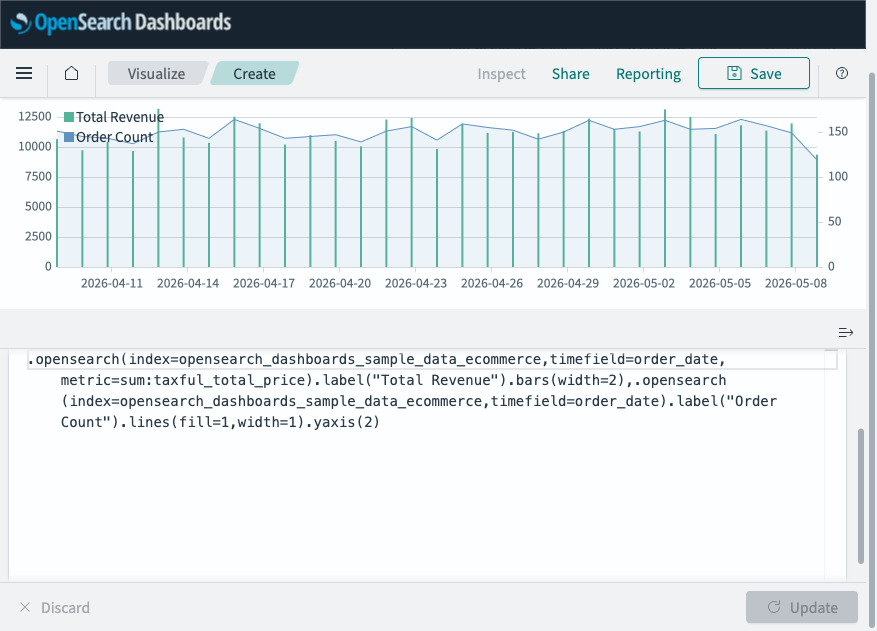
The following expression displays revenue as bars on the left y-axis and order count as a line on the right y-axis:
.opensearch(index=opensearch_dashboards_sample_data_ecommerce, timefield=order_date, metric=sum:taxful_total_price).label("Total Revenue").bars(width=2),
.opensearch(index=opensearch_dashboards_sample_data_ecommerce, timefield=order_date).label("Order Count").lines(fill=1, width=1).yaxis(2)
The following image shows the dual y-axis visualization with revenue as bars and order count as a line.
Data transformation functions
Data transformation functions modify, smooth, or analyze series data.
.movingaverage()
Calculates the moving average over a given window. Use this function to smooth noisy series. Aliases: .mvavg(). The following table lists the .movingaverage() function parameters.
| Parameter | Type | Description |
|---|---|---|
window | Number or String | The number of points, or a date math expression (for example, 1d or 1M) to average over. |
position | String | The position of the averaged points relative to the result time. One of left, right, or center. |
Example
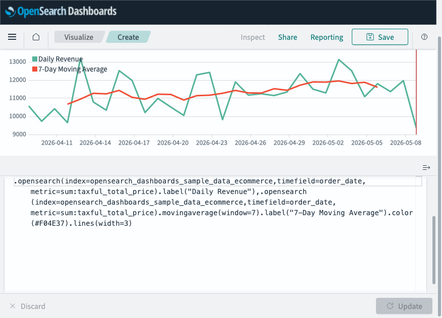
The following expression overlays daily revenue with a 7-day moving average:
.opensearch(index=opensearch_dashboards_sample_data_ecommerce, timefield=order_date, metric=sum:taxful_total_price).label("Daily Revenue"),
.opensearch(index=opensearch_dashboards_sample_data_ecommerce, timefield=order_date, metric=sum:taxful_total_price).movingaverage(window=7).label("7-Day Moving Average").color(#F04E37).lines(width=3)
The following image shows daily revenue with a 7-day moving average overlay.
.movingstd()
Calculates the moving standard deviation over a given window. Aliases: .mvstd(). The following table lists the .movingstd() function parameters.
| Parameter | Type | Description |
|---|---|---|
window | Number | The number of points to compute the standard deviation over. |
position | String | The position of the window slice relative to the result time. One of left, right, or center. Default is left. |
Example
The following expression calculates the 5-point moving standard deviation:
.opensearch(index=opensearch_dashboards_sample_data_ecommerce, timefield=order_date).movingstd(window=5).label("5-Point Std Dev")
.derivative()
Plots the change in values over time.
Example
The following expression plots the change in order count over time:
.opensearch(index=opensearch_dashboards_sample_data_ecommerce, timefield=order_date).derivative().label("Change in Order Count")
.trend()
Draws a trend line using a specified regression algorithm. The following table lists the .trend() function parameters.
| Parameter | Type | Description |
|---|---|---|
mode | String | The algorithm to use. One of linear or log. |
start | Number | Where to start calculating. Negative values count from the end. Default is 0. |
end | Number | Where to stop calculating. Negative values count from the end. Default is 0. |
Example
The following expression overlays a linear trend line on the order count:
.opensearch(index=opensearch_dashboards_sample_data_ecommerce, timefield=order_date).label("Order Count"),
.opensearch(index=opensearch_dashboards_sample_data_ecommerce, timefield=order_date).trend(mode=linear).label("Trend").color(#E53935)
.cusum()
Returns the cumulative sum of a series, starting at a base value. The following table lists the .cusum() function parameters.
| Parameter | Type | Description |
|---|---|---|
base | Number | The number to start at. This value is added to the beginning of the series. |
.fit()
Fills null values using a defined fit function. The following table lists the .fit() function parameters.
| Parameter | Type | Description |
|---|---|---|
mode | String | The algorithm to use. One of average, carry, nearest, none, or scale. |
.trim()
Sets N buckets at the start or end of a series to null. Use this function to address the partial bucket issue. The following table lists the .trim() function parameters.
| Parameter | Type | Description |
|---|---|---|
start | Number | The number of buckets to trim from the beginning. Default is 1. |
end | Number | The number of buckets to trim from the end. Default is 1. |
Mathematical functions
Timeline supports the following mathematical functions for combining or transforming series. Mathematical functions accept either a number or another series as an argument.
| Function | Description |
|---|---|
.add() (aliases: .plus(), .sum()) | Adds the values of one or more series to each position in the input series. |
.subtract() | Subtracts the values of one or more series from each position in the input series. |
.multiply() | Multiplies the values of one or more series at each position in the input series. |
.divide() | Divides the values of one or more series at each position in the input series. |
.abs() | Returns the absolute value of each value in the series. |
.log() | Returns the logarithm of each value (default base: 10). |
.min() | Returns the minimum value between the current and the provided series or number at each position. |
.max() | Returns the maximum value between the current and the provided series or number at each position. |
.precision() | Truncates the decimal portion of values to the specified number of digits. |
.scale_interval() | Scales a value (usually a sum or a count) to a new interval, for example, a per-second rate. |
.range() | Changes the maximum and minimum of a series while keeping the same shape. |
Example
The following expression calculates revenue per order by dividing the total revenue by the order count:
.opensearch(index=opensearch_dashboards_sample_data_ecommerce, timefield=order_date, metric=sum:taxful_total_price).divide(value=.opensearch(index=opensearch_dashboards_sample_data_ecommerce, timefield=order_date)).label("Revenue per Order")
Conditional function
Use the conditional function to set values based on comparison logic.
.condition()
Compares each point to a number or the same point in another series using an operator, then sets its value to the result if the condition proves true. If else is omitted, points that do not meet the condition retain their original value. Aliases: .if(). The following table lists the .condition() function parameters.
| Parameter | Type | Description |
|---|---|---|
operator | String | The comparison operator: eq, ne, lt, lte, gt, or gte. |
if | Number or SeriesList | The value to compare each point against. |
then | Number or SeriesList | The value to set if the comparison is true. |
else | Number or SeriesList | The value to set if the comparison is false. |
Example
The following expression caps values at 150 and sets lower values to 0:
.opensearch(index=opensearch_dashboards_sample_data_ecommerce, timefield=order_date).condition(operator=gte, if=150, then=150, else=0).label("Days Meeting Target")
Static values
Use static values to draw reference lines, such as targets or thresholds, on your chart.
.static()
Draws a single value as a horizontal line across the chart. Aliases: .value(). The following table lists the .static() function parameters.
| Parameter | Type | Description |
|---|---|---|
value | Number or String | The single value to display. You can pass several values to interpolate them evenly across the time range. |
label | String | The label for the series. |
offset | String | Offsets the series retrieval by a date expression. |
fit | String | The algorithm to use for fitting. One of average, carry, nearest, none, or scale. |
Example
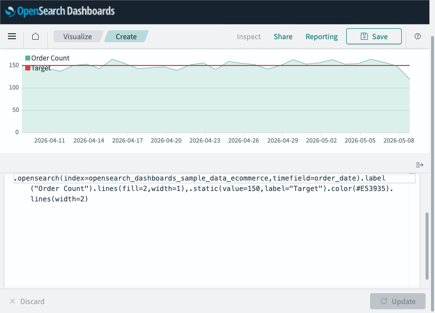
The following expression adds a target line at 150 orders:
.opensearch(index=opensearch_dashboards_sample_data_ecommerce, timefield=order_date).label("Order Count").lines(fill=2, width=1),
.static(value=150, label="Target").color(#E53935).lines(width=2)
The following image shows the order count with a static target line at 150 orders.
Aggregation function
Use the aggregation function to reduce a series to a single value and display it as a horizontal line.
.aggregate()
Creates a static line based on the result of processing all points in the series. The following table lists the .aggregate() function parameters.
| Parameter | Type | Description |
|---|---|---|
function | String | One of avg, cardinality, min, max, last, first, or sum. |
Example
The following expression displays the order count with its average as a horizontal line:
.opensearch(index=opensearch_dashboards_sample_data_ecommerce, timefield=order_date).label("Order Count"),
.opensearch(index=opensearch_dashboards_sample_data_ecommerce, timefield=order_date).aggregate(function=avg).label("Average").color(#E53935)
Forecasting function
Use the forecasting function to predict future values based on historical patterns in your series.
.holt()
Samples the beginning of a series and uses it to forecast future values using Holt-Winters triple exponential smoothing. Use this function for anomaly detection. Null values are filled with forecasted values. The following table lists the .holt() function parameters.
| Parameter | Type | Description |
|---|---|---|
alpha | Number | The smoothing weight from 0 to 1. Higher values make the series follow the original more closely. |
beta | Number | The trending weight from 0 to 1. Higher values make rising or falling lines continue longer. |
gamma | Number | The seasonal weight from 0 to 1. Higher values give recent seasons more importance. |
season | String | The season length, for example, 1w for weekly patterns. Only useful with gamma. |
sample | Number | The number of seasons to sample before predicting. Only useful with gamma. Default is all. |
Example
The following expression forecasts order count using Holt-Winters smoothing:
.opensearch(index=opensearch_dashboards_sample_data_ecommerce, timefield=order_date).label("Actual"),
.opensearch(index=opensearch_dashboards_sample_data_ecommerce, timefield=order_date).holt(alpha=0.5, beta=0.5).label("Forecast").color(#E53935)
Next steps
- To choose a different visualization type, see Choosing a visualization type.
- To add this visualization to a dashboard, see Creating dashboards.